
Appendix B: Application of satellite remote sensing to soil quality assessment - James Nuttall
Back to: Soil health for Victoria's agriculture - context, terminology and concepts
Introduction
Plant growth and water use provide an integrated measure of soil quality, taking into account soil physical, chemical and biological factors over the entire soil profile. Measuring plant growth, using biomass estimates and water use is relatively inexpensive compared with edaphic characterisation. From a grower perspective, crop yield and input costs are prime indicators for sustainability, where production is likely to influence management decision made by growers. Plant Biomass is potentially a robust indicator of soil quality for the following reasons:
1. it integrates soil physical, chemical, and biological condition,
2. it encompasses the soil profile within the effective rooting zone
3. it is linked closely to gross margin thus has grower incentive to measure, and
4. it is readily measurable. For agricultural production systems the challenge exists in relating point source quantitative analyses of soil quality to broader scale ecosystem process of sustained crop growth and production.
Measurement of biomass can be made over a range of scales from point source to regional level using sensors mounted on vehicles, airborne and satellite platforms. Vehicle and airborne mounted sensors serve intra, inter–paddock purpose of crop assessment such as canopy management in precision agriculture. In contrast satellite platforms tend towards large–scale appraisal of landscape systems, thus suitable for assessment of spatial and temporal variation of vegetation across a broad area. As this review focuses on soil quality and capacity to support production systems at an ecosystem scale then discussion will focus on satellite derived vegetation indices.
Satellite–derived information for estimating crop production has been well established. In particular the Advanced Very High Resolution Radiometer (AVHRR) installed on the National Oceanic and Atmospheric Administration (NOAA) suite of satellites has been used to analyse agricultural systems. Applications include crop forecasting (Maselli, 1992; Quarmby, 1993; Benedetti, 1993; Smith, 1995), crop water dynamics studies (Veron, 2002) assessing ecosystem service (Prince, 1986; Konarska, 2002; Lu, 2003) soil mapping (Dobos, 2000) and climate (Kerr, 1989). For NOAA–AVHRR the limited spatial resolution of the sensors means these data are best suited to large–scale appraisal of landscape systems however, paddock scale assessment is not practical (possible). Alternatively, sensors on Landsat and SPOT provide higher resolution information making them well suited to assessing impact of human activity to agricultural production from paddock to regional scale. These remote sensing techniques can potentially detect where agricultural activity has caused a shift in production potential due to changing soil quality. Alternatively in regions where open cut mining has occurred on agricultural land, satellite derived information may offer a way of determining the effectiveness of mine rehabilitation, where historical and post–mining biomass production information is compared. This would provide assessment of the long–term impact of mining on soil quality.
Satellite and sensor capability
Satellite base spectrometers measure reflectance from terrestrial features where the sensors collect information cumulated from an instantaneous field of view (IFOV) snap shots, where IFOV differs depending on sensor capability. Consecutive IFOV are taken as the satellite traverses it orbit typically ca 98.9 degrees, 8.9 degrees offset from N–S. Each snap shot represent a scene, which constitutes layers of simultaneous matrices made up of elements (pixels) each recording a reflectance values. Reflectance values are recorded using digital numbers (DN). Each simultaneous matrix represents different wavelength interval collected by the sensor. The DN’s are transformed to range from 0 to 255 where increasing number represent higher reflectance (Frank, 1985).
Reflectance data recorded from satellites range widely, depending on age and capability of sensors and orbit path (Lillesand, 1994). There are three main satellite programs, NOAA (National Oceanic and Atmospheric Administration), Landsat (formally ERTS (Earth Resources Technology Satellites)) and SPOT (Systeme Pour l’Observation de la Terre) which all have a sun–synchronous orbit (Figure 1). These satellites track westward with successive north–south orbits thus maintaining the equivalent sun angle incidence on each pass of the equator and so comparable surface illumination. Irrespective, time of year and global position impact on the suns angle of incidence and so reflectance characteristics of terrestrial features. Satellite pass frequency, off-nadar angle and cloud cover also impede comprehensive data collection.
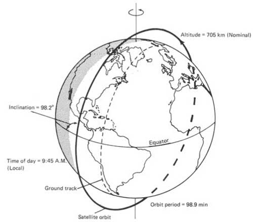
Figure 1 Sun-synchronous orbit of Landsat-4 and -5 after (Lillesand, 1994)
For the satellites, NOAA, Landsat and SPOT, their orbit characteristics are similar, however, difference in on–board sensor design control characteristics such as orbit repeat period and resolution and so variation in monitoring capability. NOAA AVHRR has a wide scan angle compared with Landsat TM and SPOT HRV consequently coverage repetition is shorter (8–9 days) thus providing high temporal resolution. This high temporal resolution allows correction for cloud cover where successive overpasses for a discrete period are combined and the maximum reflectance taken for each grid point (Holben 1986; Smith 1995; Benedetti 1993). Conversely, AVHRR low spatial resolution (1100 × 1100 m) limits it application to paddock scale studies. For Landsat TM (30 × 30 m) and SPOT (20 × 20 m) their sensitivity is suited to monitoring paddock scale processes, although their lower temporal resolution gives less control over noise filtering due to factors such as cloud cover. For example, data estimating wheat crop distribution and yields in NSW, from Landsat was 57% cloud affected for paddock assessed around anthesis (Dawbin, 1980). Assessment of vegetation cover in south central Utah was also complicated by reduced temporal resolution of data due to cloud (Ramsey, 2004) and again estimation of wheat cover in Kansas and Indiana was hindered by cloud cover (Bauer, 1977). Despite these potential draw backs, data from Landsat based sensors appear the best option for assessing temporal/spatial change in soil quality, through remotely derived vegetation indices.
Table 1. Comparison of current satellites and sensors. TM*, spatial resolution for the thermal–IR band is 120m. ETM+ spatial resolution is 60 m in thermal band and a 15 m panchromatic band.
Parameter | Satellites | ||
Landsat -5. -7 | SPOT -1, -2, -3 (4&5) | NOAA -7, -9, -11 | |
| Altitude (m) | 900 | 832 | 833 |
| Orbit time (m) | 103 | 102 | |
| Orbit inclination (degrees) | 98.2 | 98.7 | 98.9 |
| Orbits per day | 14.5 | 14.1 | |
| Orbit repeat period (days) | 16/18 (offset 8) | 26 | 8-9 |
Sensors | |||
MMS, TM & EM+ | HRV x 2 | AVHRR | |
| Scan angle from nadir (degrees) | 7.7 - TM | variable up to 27 | 55.4 |
| Swath width (km) | 185 | 80 to 117 | 2400 |
| Scene (FOV) (ha) | |||
| Resolution (m) | 30 - TM* 80 - MSS | 10 - panchromatic 20 - multispectral | 1100 |
| Cost (scene ) | $600 (US) | ||
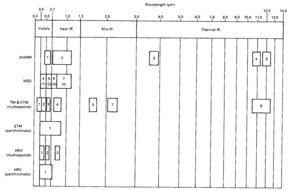
Figure 2. Spectral sensitivity of AVHRR, MSS, TM&ETM and HRV (Lillesand, 1994)
Landsat coverage
The coverage of Landsat is defined by the world reference system (WRS). The WRS is a grid overlaid on the earth surface made up of 233 near vertical paths, numbered consecutively from east to west, which relate to the ground track of the satellite. Path 001 intersects the equator at 64.60ο west longitude and consecutive swaths overlap. The horizontal (latitudinal) portion of the grid is defined by rows (1 to 122), which provide the interval at which scenes are captured. Scenes are identified by the nomenclature 195/028, where path number is listed first, and the intersection of the path and row define the centre point of a single scene (Figure 3) (Anon, 2006b).
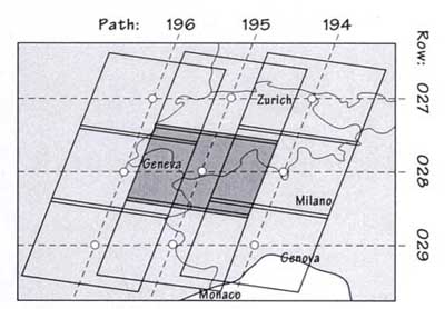
Figure 3. (Anon, 2006b)
Although a standard full scene (170 × 185 km) covers a prescribed portion of ground, several options exist in the acquisition of Landsat data. Within Australia, the Australian Centre for Remote Sensing (ACRES) – http://www.ga.gov.au/acres/ (external link) supply these data. Apart from purchasing a full standard scene, floating full scenes and portions of single scenes are available, where floating scenes constitute portions of several scenes. Portions of single scenes (eg quarter scene) are also based on the standard and floating options (Anon, 2006b). These variations relate to geometric manipulation of data, see ‘data processing’.
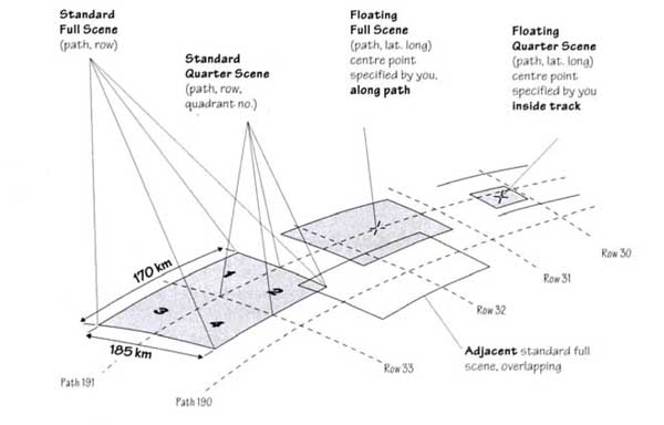
Figure 4. (Anon, 2006b).
Data Processing
Information from satellite sensors is received as a sequential stream of pixel data, which requires reconfiguring into a useable format. The degree of processing varies depending on what the end user requires. Typically processing level falls into two categories, level 0 and 1. Level 0 (0R) constitutes raw data that has not had radiometric noise removed and are not geometrically corrected. Data in this format requires substantial manipulation by the end user. In contrast level 1 data has correction applied for either radiometric (1R) or radiometric/geometric factors (1G). Raw data supplied by ACRES is equivalent to the United States Geological Survey (USGS) 1R level, which has radiometric correction.
Radiometric calibration
Radiometric correction removes/minimises effects due to impulse noise, and recalculates band reflectance as integer values. Within this manipulation there is the standardization of radiances across detectors. This is required as satellites carry multiple detectors within each band that vary in their compliance. As these detectors operate simultaneously to produce scenes where scan lines are compiled from multiple sensors, brightness values of adjacent scan lines vary, producing images that are stripped in the across track direction (Anon 2006a). Relative radiometric correction removes this effect by correcting brightness values using a reference standard. This standard is either taken from a nominated single reference detector, or by taking the mean brightness values across all detectors and correcting to this. Alternatively the multiple detectors within each band are individually corrected using time–dependent calibration algorithms (look up tables (LUT)). ACRES (Geoscience Australia) provide data that has been radiometrically corrected. For Landsat 5 TM data this is corrected in bands 1, 2, 3, 4, 5 and 7 using LUT and band 6 (thermal) using across detector averages. (Anon 2006a).
Geometric correction
Geometric correction realigns pixel data into a spatial context. Within this conversion, several factors have to be accounted for which include sensor operation, satellite orbit and terrestrial characteristics. Terrestrial variables are earths rotation and curvature. Spatially the data can be reconstructed as path or map orientated product. For path orientated data, the map grid is aligned with the satellite path (ca. 10O east of north) and is not compatible to GIS applications. Alternatively, the data can be manipulated to align with map–grid north. A relic of the resampling process is a reduction in pixel size from 30 × 30 metres to 25 × 25 metres. ACRES supply both path and map orientated data where projection format is the Australian Geodetic datum of 1966 (AGD 66). These data are not corrected for atmospheric effects such as cloud cover (Anon, 2006b).
Registering the map grid to actual terrestrial position involves either a systematic or precision correction (Anon 2006a). The systematic correction relies on theoretical calculation of position using satellite trajectory information. In contrast, the precision correction (ortho–corrected) uses ground control points (GCP) for more accurate grid to terrestrial registration. Historically ACRES, Australia assigned GCP using topographic maps, however, more recently GCP have been redefined using geo–coded image chips, calibrated from controlled passes of Landsat ETM+ (Wang). Assessment of these orthocorrected products indicates that absolute positional accuracy is between 7 and 13 metres (< 0.5 pixel). This infers that multi–temporal, sub–pixel registration is possible, which potentially provides the capacity to make temporal assessment of land systems on a paddock scale. Ortho–corrected products are routinely available form ACRES for Australian coverage. Table 2 gives costs of sourcing Landsat data for Australia coverage which depends on scene size and degree of data manipulation required.
Table 2. Cost and scene size for satellite data.
Satellite/Sensor | Scene size | Cost (A$) |
Landsat 7/ETM+ Landsat5/TM | 25 x 25 km | 450-550 |
| 60 X 60 Km | 670-770 | |
| 90 X 90 Km (quarter scene) | 860-960 | |
| 130 x 1130 km (half scene) | 1100-1200 | |
| 185 x 170 (full scene) | 1500-1800 | |
| Double scene | 2000-2200 | |
| Triple scene | 2600-2800 | |
| Landsat5/MSS | 185 x 170 km (full scene) | 595 |
Vegetation Indices
Remote sensing techniques can be used for monitoring vegetation (Lillesand, 1994). Numerous satellite systems measure reflectance in the optical spectrum, which includes the ultraviolet, visible, near–, mid–, and thermal infrared wavelengths (0.3–14 μm). Specifically bands in the visible and near infrared region can be used to derive various vegetation indices. The link between radiation reflectance from transpiring leaves and growth occurs due to the surface structure of leaves attenuating radiation in the red visible and near infrared bands. When solar radiation incorporating the visible and near infrared range (0.4 – 1.5 μm) hit transpiring leaves internal scattering of frequencies occurs. Radiation in the 0.4 –0.7 μm (red) range is heavily absorbed by the leaf chlorophyll whereas little absorption occurs in the 0.7 –1.3 μm near infrared range (Tucker, 1986). A common index used to define plant growth and biomass production, based on this principal, is the normalized difference vegetation index (NDVI). This is a ratio of the difference between the red (0.63–0.69 μm) and near infrared (0.76–0.90 μm) and their sum i.e.
Where, the index relates to the plants photosynthetic efficiency (Tucker, 1986). Alternative indices are also simple ratios (SR) of NIR and red bands (Lobell, 2001) or their difference (difference vegetative index (DVI)) (Anderson, 1993).
1. Differentiating ground cover
Early example using Landsat MSS was identifying and making area estimation of winter wheat in Kansas (Bauer, 1977), found good agreement between Landsat and United States Department of Agriculture statistics. Other applications of reflectance data from Landsat MSS were differentiating between degree and type of ground cover in semi–arid regions. (Frank, 1985) showed that reflectance band ratios could differentiate between halophytic shrubs, perennial grasses, shrubs and forest stands in Utah, USA using growth rate, where successive images were compared over a 2–month period. Similarly (Dawbin, 1980) showed that temporal comparison of radiance, from Landsat MSS, over a 3–month period during the wheat–growing season could discriminate between wheat, pasture and fallow paddocks in agricultural regions of New South Wales, Australia. In contrast assessing area of corn and soybean crops in Indiana using MSS was less successful due to crops being spectrally similar to other cover types (trees) and the smaller paddock size being beyond the spatial resolution of these sensors. Alternative cover indexes have also been used to monitor change in vegetation cover over time (Pickup et al. 1993). These workers used Landsat MSS scenes from over arid rangeland in Alice Springs, where the index was designed to differentiate between bare earth and vegetation cover. They used Band–4/band–5 data space to define an upper soil line (limit) and calculated the relative perpendicular position (PD54) of individual pixels to this line. This index showed better agreement with percent vegetation cover under dry and wet conditions than NDVI. For monocultures, however, it is likely that the NDVI will be a superior index as it has high greenness sensitivity implied better predictor of variation in crop biomass within paddock.
2. Assessing crop production
Reflectance measurements can be used to estimate crop yield by linking amount of photosynthetically active radiation absorbed by the crop canopy to biomass production. Prediction of wheat yields in north–western NSW was made using Landsat MSS where temporal difference in reflectance data was calculated between early emergence and maturity. For two combinations of bands, a log transformed (log10) ratio of bands 7 and 5 (near–infrared/red) best fit observed wheat yield. Landsat 7 (ETM+) imagery could also accurately predict wheat yield at both the regional and local scale in Sonara, Mexico (Lobell, 2001) using a light–use efficiency estimated by the simple ratio (SR) and NDVI. This methodology overcomes atmospheric effects and the need for extensive ground truthing compared with models that rely on leaf area indices (Lobell, 2001). In shrub-steppe environments in south–central Utah, vegetation cover was also estimated using Landsat ETM where the NDVI had superior agreement with vegetation abundance compared with single band reflectance data (Ramsey, 2004). For growth of short grass prairie in central plains of northeast Colerado three vegetation indices were tested against three methods of combining spectral data from Landsat TM and biomass production. For univariate models, best agreement existed between green biomass and NDVI, when biomass data was combined into greenness strata prior to registration with reflectance data (Anderson, 1993). Reflectance information was also used in phenological studies of crop (Boissard, 1993), where NDVI was strongly linked to ear water concentration in wheat after anthesis and crop developmental stage, allowing for forecasting of crop maturity times. Overall, of the various possible reflectance channels and indices, the NDVI appears the most robust in estimating photo–synthetically active vegetation within a growing season.
3. Assessing change in soil quality
Using Landsat MSS, Frank (1985) (Frank, 1985) demonstrated that registration of pixels across successive images using simple regression could identify change in land quality (deviation from x=y) in a semi–arid environment after thunderstorm events. In this case reflectance information was sensitive to vegetation productivity and erosion process over a 2–month period in Utah, USA, where the region was uniformly exposed to thunder storm events. This approach demonstrates the capacity to monitor small–scale change in land quality, however, varying seasonal condition across the landscape may complicate its application to large regions (Frank, 1985). In contrast (Anderson, 1993), who was using Landsat TM data to monitor short prairie grass on semi arid central plains in east Colerado, found a poor correlation with vegetation indices when direct sample point to pixel (or aggregated pixels) were used. These workers contributed this to inability to accurately register pixels to sample points. The other difficulty is deciding if the change is due to management factors, natural variability of physical processes or both.
Proposed methodology for assessing change in soil quality
When assessing soil quality in agricultural zones, it is assumed that the main ecosystem service associated with the soil resource is the potential to support biomass production. Logically if, the capacity of soil to sustain production changes then this implies a change in soil quality. The challenge is to use crop biomass estimates to identify those parts of the landscape that are fluxing in production stability. Although numerous applications of satellite derived data attempts to make quantitative measurement for crop yield forecasting purposes etc, estimating change in soil quality is more one of assessing temporal change in production for any one point (pixel) within the landscape. For example within a single paddock regions may be consistently low or high yielding (stable) or alternatively show temporal switching tendencies where yield from year to year is variable, all of which would not suggest any fundamental change in soil quality but relate more to intrinsic/static soil quality. To demonstrate a shift in soil quality there needs to be a change in stability. If parts of the paddock/landscape become more/less stable this may infer there has been a shift in capacity of the soil to support growth of vegetation and so change in soil quality. Ideally at an intra–paddock level if the paddock could be divided up into a grid based on sensor resolution and registration accuracy, then temporal change of these individual blocks could be tracked.
For Landsat sensors with 30 × 30 metres resolution and ortho–corrected data being sub–pixel in absolute position accuracy, then it is possible to have accurate multi–temporal registration of pixels on a 30 metres grid. Alternatively, to decrease overlap error, pixels could be grouped eg 2 × 2 or 3 × 3, where the average radiance values of these is used. Once multi–temporal data, spanning 5 to 10 years is acquired and grid points are registered then each layer will require standardisation to allow for difference in range of absolute radiance data for each year, associated with different biomass potential across crops. This standardized data could be used to infer stability of biomass production relative to the paddock mean at any point within the paddock.
The output is likely to fall into one of three categories, which include, a). areas that are consistently high or low yielding, this would relate to potential inferred by intrinsic soil quality, b). portions of the paddock which are show temporal switching (unstable) which relates to interaction of intrinsic soil quality, season climatic conditions and crop type and c). parts of the paddock which have a negative trend, which implies a shift in soil capability to support plant growth and thus a potential shift in soil quality. A simplistic example could be the gradual expansion of saline land in a discharge zone, which is expressed as a gradual reduction in plant growth, radiating out form the saline source.
The information could be expressed either spatially in a map format where the various zones are identified. Alternatively, the multi–temporal reflectance data, after standardisation, could be divided into percentiles for each year. The distribution of these percentiles could then be compared across years. A shift in distribution of biomass with time would indicate changing status of soil quality.
Indices used
1. (Bauer, 1977) Landsat MSS
- Green = Band4
- Red = Band5
- NIR1 = Band6
- NIR2 = Band7
2. (Dawbin, 1980) Landsat MSS
- Green = Band4
- Red = Band5
- NIR1 = Band6
- NIR2 = Band7
- 10log10(100 × NIR2/Red) = 10log10(100 × Band7/Band5)
3. (Frank, 1985) Landsat MSS
- Green = Band4
- Red = Band5
- NIR1 = Band6
- NIR2 = Band7
4. (Anderson, 1993) Landsat TM
- DVI (difference vegetative index) = NIR – Red = Band4–Band3
- RVI (ratio vegetative index) = NIR/Red = Band4/Band3
- NDVI = (NIR – Red)/(NIR + Red) = (Band4 – Band3)/(Band4 + Band3)
5. (Pickup, 1993) Landsat MSS where band 4 = green, band 5 = red, band 6 = near IR and band 7 =near/mid IR
- Red = Band5
- NDVI = (NIR2 – Red)/(NIR2 + Red) = (Band7 – Band5)/(Band7 + Band5)
- SSI (soil stability index) = perpendicular distance of each pixel from the soil line in band4/band7 and band 5/band 7 data space
- D54 = perpendicular distance of each pixel from the upper soil line (upper soil band limit) in the band 4 and band 5 data space.
6. (Boissard, 1993) SPOT HRV
- NDVI = (NIR – Red)/(NIR + Red) = (Band4 – Band3)/(Band4 + Band3)
7. (Lobell, 2001) Landsat ETM+
- SR (simple ratio) = NIR/Red = Band4/Band3
- NDVI = (NIR – Red)/(NIR + Red) = (Band4 – Band3)/(Band4 + Band3)
8. (Ramsey, 2004) Landsat ETM
- Blue = Band1
- Green = Band2
- Red = Band3
- NIR = Band4
- MIR1 = Band5
- MIR2 = Band7
- NDVI = (NIR – Red)/(NIR + Red) = (Band4 – Band3)/(Band4 + Band3)
References
Anderson GL, Hanson JD, Haas RH (1993) Evaluating landsat thematic mapper derived vegetation indices for estimating above–ground biomass on semiarid rangelands. Remote Sensing of Environment 45, 165–175.
Anon (2006a) Australian Government. In 'Geoscience Australia'. (www.ga.gov.au/acres) (external link)
Anon (2006b) Eurimage – Landsat. In. (www.eurimage.com) (external link)
Bauer ME, Hixson MM, Davis BJ, Etheridge JB (1977) Crop indentification and area estimation by computer–aided analysis of landsat data. Machine Processing of Remotely Sensed Data Symposium, 102–112.
Benedetti R, Rossini P (1993) On the use of NDVI profiles as a tool for agricultural statistics: The case study of wheat yield estimate and forecast in Emilia Romagna. Remote Sensing of Environment 45, 311–326.
Boissard P, Pointel JG, Huet P (1993) Reflectance, green leaf area index and ear hydric status of whear from anthesis until maturity. International Journal of Remote Sensing 14, 2713–2729.
Dawbin KW, Evans JC, Duggin MJ, Leggett EK (1980) Classification of wheat areas and prediction of yields in north–western New South Wales by repetitive landsat data. Australian Journal of Agricultural Research 31, 449–453.
Dobos E, Micheli E, Baumgardner MF, Biehl L, Helt T (2000) Use of combined digital elevation model and satellite radiometric data for regional soil mapping. Geoderma 97, 367–391.
Frank TD (1985) Remote sensing land quality changes in arid and semiarid environments: a review. Annals of Arid Zone 24, 211–217.
Holben BN (1986) Characteristics of maximum–value composite images from temporal AVHRR data. International Journal of Remote Sensing 7, 1417–1434.
Kerr YH, Imbernon J, Dedieu G, Hautecoeur O, Lagouarde JP, Seguin B (1989) NOAA AVHRR and its uses for rainfall and evaporation monitoring. International Journal of Remote Sensing 10, 847–854.
Konarska KM, Sutton PC, Castellon M (2002) Evaluating scale dependence of ecosystem service valuation: a comparison of NOAA–AVHRR and Landsat TM datasests. Ecological Economics 41, 491–507.
Lillesand TM, Kiefer RW (1994) ʹRemote sensing and image interpretation.ʹ (John Wiley and Sons Inc: New York)
Lobell DB, Asner GP (2001) Regional wheat yield prediction using landsat 7 satellite imagery. Third International Conference on Geospatial Information in Agriculture and Forestry.
Lu H, Raupach MR, McVicar TR, Barrett DJ (2003) Decomposition of vegetation cover into woody and herbaceous components using AVHRR NDVI time series. Remote Sensing of Environment 86, 1–18.
Maselli F, Conese C, Petkov L, Gilabert MA (1992) Use of NOAA–AVHRR NDVI data for environmental moitoring and crop forecasting in the Sahel. Preliminary results. International Journal of Remote Sensing 13, 2743–2749.
Prince SD, Tucker CJ (1986) Satellite remote sensing of rangelands in Botswana II. NOAA AVHRR and herbaceous vegetation. International Journal of Remote Sensing 7, 1555–1570.
Quarmby NA, Milnes M, Hindle TL, Silleos N (1993) The use of multi–temporal NDVI measurements from AVHRR data for crop yield estimation and prediction. International Journal of Remote Sensing 14, 199–210.
Ramsey RD, Wright Jr DL, McGinty C (2004) Evaluating the use of landsat 30m enhanced thematic mapper to monitor vegetation cover in shrub–steppe environments. Geocarto International 19, 39–47.
Smith RCG, Adams J, Stephens DJ, Hick PT (1995) Forecasting wheat yield in a mediterraneantype environment from the NOAA satellite. Australian Journal of Agricultural Research 46, 113–125.
Tucker CJ, Sellers PJ (1986) Satellite remote sensing of primary production. International Journal of Remote Sensing 7, 1395–1416.
Veron SR, Paruelo JM, Sala OE, Laurenroth WK (2002) Environmental controls of primary production in agricultural systems of the Argentine Pampas. Ecosystems 5, 625–635.
Wang L–W, Smith C Accuracy assessment of ACRES landsat orthocorrected products.
© State of Victoria (Agriculture Victoria) 1996 - 2025.

This work, Victorian Resources Online, is licensed under a Creative Commons Attribution 4.0 licence. You are free to re-use the work under that licence, on the condition that you credit the State of Victoria (Agriculture Victoria) as author, indicate if changes were made and comply with the other licence terms.
The licence does not apply to ‘branding’ or some ‘images or photographs’ that may be owned by third parties. We ask you to seek prior approval to use images using the VRO feedback form. Access to higher quality images can also be provided on request.
This page was last updated on 23/03/2020.